Principle: DESeq2 is based on a negative binomial distribution model, taking into account the discreteness and variability of gene expression data, as well as the impact of library size differences on differential analysis. DESeq2 reduces technical variation between samples through normalization transformations and scaling factors, then estimates the dispersion of gene expression. It employs the negative binomial distribution model to identify differentially expressed genes and corrects for multiple testing issues. DESeq2 is suitable for small sample RNA sequencing data and performs particularly well with a small number of samples, effectively handling inter-sample variability, technical noise, and batch effects.
Input Data Type: DESeq2 is designed for RNA-seq data and requires count data for each gene. It typically uses raw count matrices without the need for pre-normalization or scaling. DESeq2 requires the input data to be a matrix composed of integers. In addition to importing counts, DESeq2 officially provides a method to directly import txi objects generated by tximport if salmon was used upstream.
edgeR(Empirical Analysis of Digital Gene Expression Data in R)
Principle: Similar to DESeq2, edgeR also accounts for the dispersion in data. It utilizes a negative binomial distribution model and different normalization methods, such as TMM (Trimmed Mean of M values), to address technical variations between samples. edgeR employs a hypothesis-testing framework to identify differentially expressed genes and uses multiple testing correction akin to the Benjamini-Hochberg method. edgeR performs better with a larger number of samples and is suitable for medium-scale RNA sequencing data, offering high sensitivity and accuracy.
Input Data Type: edgeR is also applicable to RNA-seq data, requiring expression counts for each gene. It uses the raw count matrix and does not require normalization or standardization. When using edgeR, it is important to select the appropriate analysis algorithm; the official recommendation for bulk RNA-seq is the quasi-likelihood (QL) F-test tests, and for scRNA-seq or data without replicates, the likelihood ratio test is suggested.
Group Table:
group
normal  tumor
   811    470
Change Table:
down stable up
2984 20294 3842
head(DEG_edgeR, 5)
                  logFC   logCPM        LR PValue FDR change
CH507-513H4.4 -16.46830 8.739277  9184.402      0   0   down
CH507-513H4.3 -16.18797 8.739279  8829.571      0   0   down
XBP1          -15.00117 5.932264 40023.604      0   0   down
CH507-513H4.6 -14.81025 8.739297  7042.096      0   0   down
KREMEN1       -14.45332 5.384819 22028.487      0   0   down
4.3 Performing differential analysis using limma
limma(Linear Models for Microarray Data)
Principle: Initially developed for gene chip data, limma was later adapted for RNA sequencing data. It is based on linear models and employs weighted least squares for estimating differences in gene expression, and a Bayesian approach for correcting multiple testing issues. Limma excels in handling large-scale data and is suitable for high-throughput data analysis, such as chip and large-scale RNA sequencing data, effectively controlling the false positive rate.
Input Data Type: limma is applicable to various types of high-throughput data, including chip data and RNA-seq. It requires the expression values for each gene, which can be either raw counts or already normalized values. There are two methods for differential analysis in limma: limma-trend and voom. The difference between these two methods is minimal when the sequencing depth of samples is similar, but voom has advantages when there is a significant difference in sequencing depth, hence voom is generally the preferred method for differential analysis.
Group Table:
group
normal  tumor
   811    470
Change Table:

  down stable     up
  1874  16990   1611
head(DEG_limma_voom, 5)
             logFC    AveExpr         t P.Value adj.P.Val        B change
TOMM6   -11.347906  1.6560534 -319.5710       0         0 2790.496   down
EEF1G   -11.484561  6.6305909 -218.5213       0         0 2324.291   down
XBP1    -12.063108  2.1101301 -192.0646       0         0 2162.558   down
ARL6IP4  -5.415435  4.6609716 -189.5647       0         0 2149.674   down
CMC4     -7.768105 -0.5940984 -187.1232       0         0 2129.708   down
4.4 Wilcoxon Rank-Sum Test
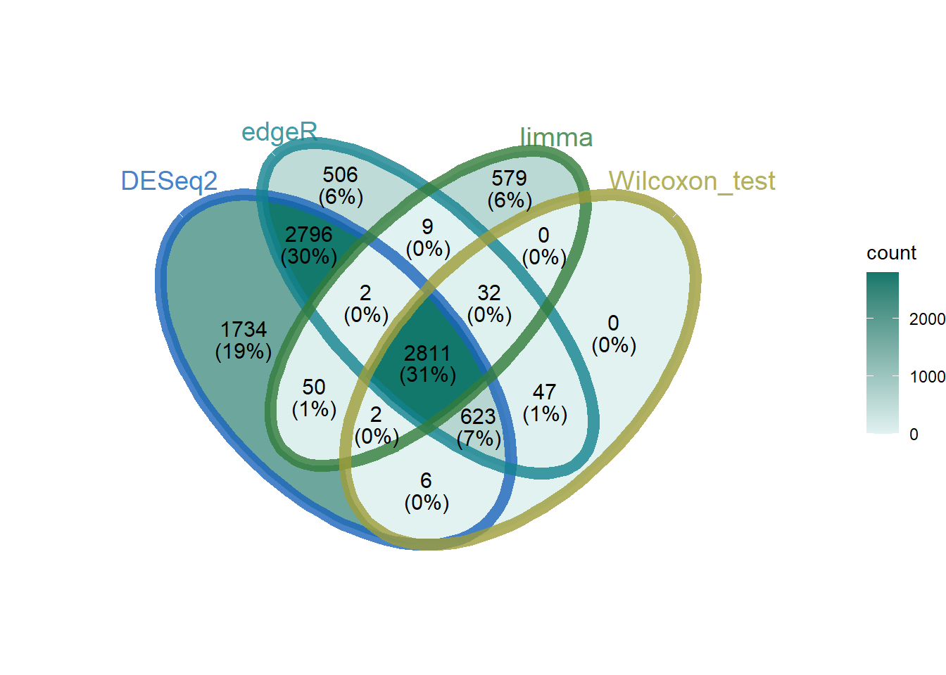
Experiments indicate that the Wilcoxon rank-sum test, as a non-parametric test, is not recommended when the sample size per condition is less than eight. However, once the sample size per condition exceeds eight, the Wilcoxon rank-sum test performs comparably or better than the three parametric testing methods (DESeq2, edgeR, and limma-voom) or other non-parametric testing methods.
The three parametric testing methods DESeq2, edgeR, and limma were all initially developed to address the problem of analysis with small sample sizes. In population-level studies, which typically have larger sample sizes (at least several dozen), parametric assumptions are often unnecessary. Additionally, larger sample sizes are more likely to include several outliers that, when they violate assumptions, can lead to unstable p-values and consequently invalidate FDR.
Unlike DESeq2, edgeR, and limma, the Wilcoxon rank-sum test, as a non-regression method, cannot adjust for various potential confounding factors (such as differences in sequencing depth). To use the Wilcoxon rank-sum test, it is generally recommended that RNA-seq samples first be normalized to eliminate batch effects before computation.
Note: The method selected for function implementation in this section is: edgeR TMM + wilcox.test analysis